The previous section introduced quantitative trading tools and basic research. This article covers the practical implementation of quantitative trading strategies and their performance.
By writing trading strategies using GPT-4.0, you can enter the financial programming field at zero cost. If the results are not ideal, you can also have it analyze the tabular files returned by the Interactive Brokers API to optimize parameters (watch out for overfitting).
Disclaimer: The following is based on my personal research, and the code was generated by GPT. It does not constitute any investment advice. Please invest with caution.
Personal Repository
Quick Start
Register an Interactive Brokers account and download Gateway
Install the backtrader library (quantitative backtesting framework)
Install the ib_insync library (for interfacing with Interactive Brokers Gateway; the developer erdewit passed away on March 11, 2024, RIP)
Write a sample SMA strategy using the ib_insync documentation or GPT
Run and observe the charts
Recommended Common Frameworks
backtrader is a traditional strategy framework. Rather than diving into AI hype right away, I prefer to master traditional frameworks first. Developed by a German programmer, its code style, structure, and design are very suitable for learning.
qlib AI quantitative framework
IB Gateway Integration
1 | import backtrader as bt |
SMA Strategy
Introduction
SMA (Simple Moving Average) sounds simple, as its name suggests, making it ideal for beginners to quickly run through a backtesting process.
SMA is calculated by taking the closing prices over a past period of time and averaging them.
For example, to calculate a security’s 20-day SMA, add up the closing prices of the past 20 days and divide by 20.
Similarly, to calculate a security’s 200-day SMA, add up the closing prices of the past 200 days and divide by 200.
Each data point in an SMA has equal weight. However, investors might consider recent data to be more important than older data and prefer to assign higher weight to recent prices. Therefore, they often favor another form of moving average, the EMA (Exponential Moving Average). EMA can provide a better reference when the market experiences rapid and sharp fluctuations.
Trend Identification
A security trading above its SMA is in an uptrend, while one trading below its SMA is in a downtrend.
It can also be used to identify support and resistance levels.
Crossovers
Bullish Crossovers and Bearish Crossovers
Investment strategies involving SMA generally rely on bullish crossovers and bearish crossovers.
A bullish crossover occurs when a security’s price falls below the SMA and then moves back above it. This signifies the end of a pullback and signals the start of an uptrend. Conversely, a bearish crossover signals the beginning of a pullback.
However, in a range-bound (oscillating) market, this indicator is less effective.
Golden Cross and Death Cross
A Golden Cross occurs when a short-term SMA crosses above a long-term SMA. For example, when the 50-day SMA crosses above the 200-day SMA, a Golden Cross appears, which is a bullish signal. The opposite is a Death Cross, which is a bearish signal.
When a Death Cross occurs, investors might consider temporarily pulling out of the market. (Reflecting on the pharma fund I bought—even though it had been in a Death Cross for two years, I was still stubborn enough to gamble on it…)
Code
Generated by GPT-4. Note that for simplicity, the code executes all-in buy and sell orders when a crossover occurs.
1 | class SmaCross(bt.Strategy): |
Performance
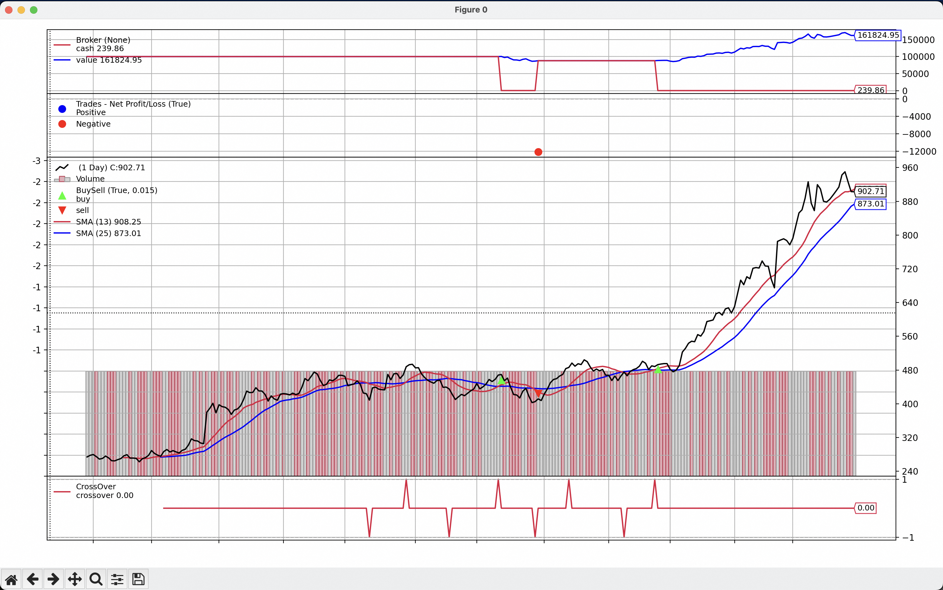
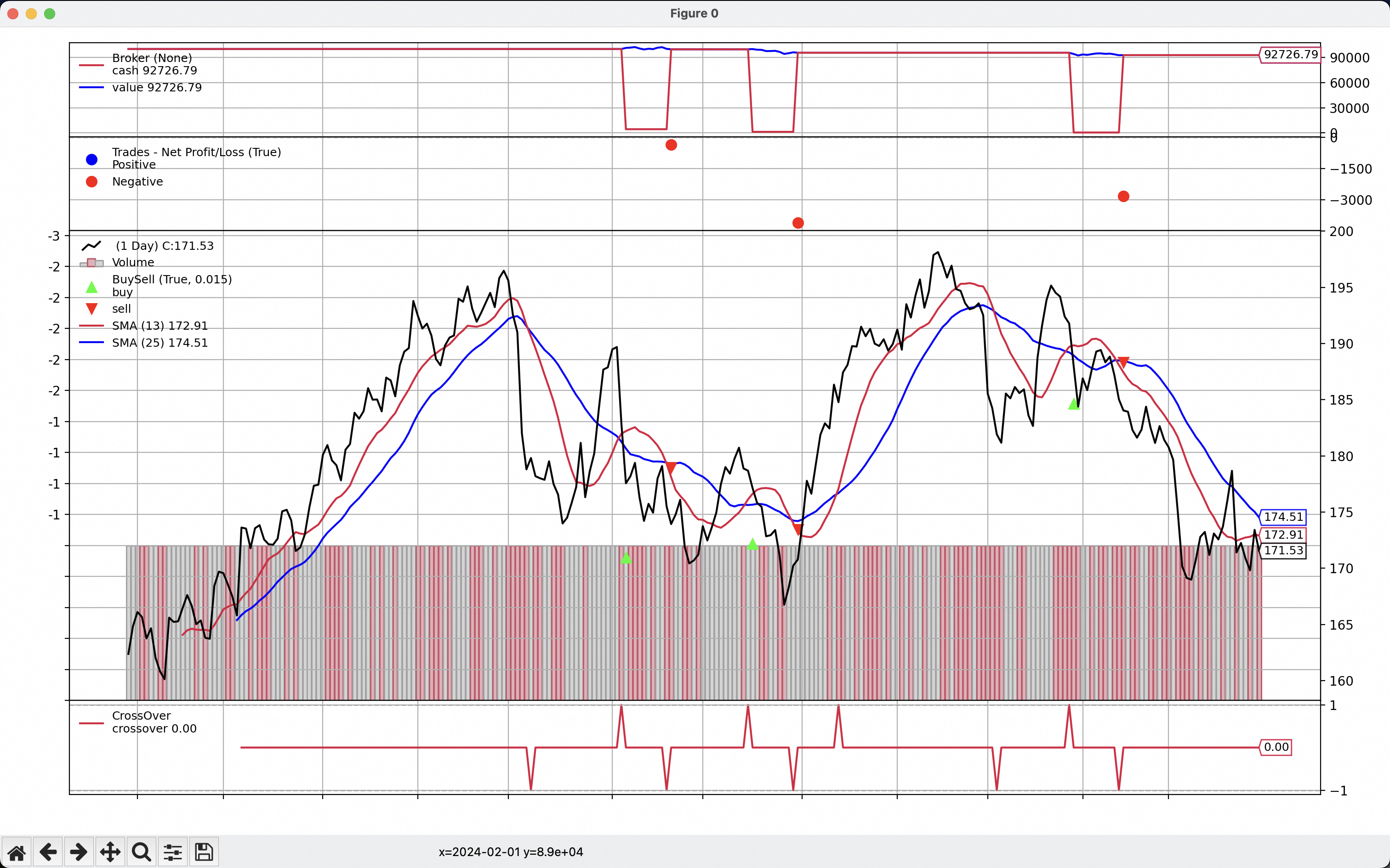
Analysis
SMA performed well on NVDA, a stock in a monotonic uptrend. NVDA rode the AI wave all the way up, but how many such hype waves are there really?
More common are fluctuating trends like AAPL’s, where SMA actually resulted in a loss of around 8%.
MACD Strategy
Introduction
MACD (Moving Average Convergence/Divergence) is known as the moving average convergence/divergence indicator. It is visible on most exchange charts and is often dubbed the King of Technical Indicators.
The MACD indicator consists of three main components: the DIF line, the DEA line, and the MACD histogram. The standard parameters are 12, 26, and 9, as shown in the code below.
- The DIF line is the fast exponential moving average (typically 12 days) minus the slow exponential moving average (typically 26 days).
- The DEA line is the 9-day weighted moving average of the DIF line.
- The MACD histogram represents the difference between the DIF line and the DEA line, used to show the degree of divergence between the DIF and DEA lines.
Crossover Strategy
The basic principle of MACD relies on golden crosses and death crosses:
- A golden cross occurs when the DIF line crosses above the DEA line, indicating strengthening bullish momentum and suggesting a potential market uptrend, which serves as a buy signal.
- A death cross occurs when the DIF line crosses below the DEA line, indicating strengthening bearish momentum and suggesting a potential market downtrend, which serves as a sell signal.
Divergence Strategy
Red/Green Bar Divergence
Red Bar Bearish Divergence: The stock price hits a new high, but the red bars fail to reach a new high. Upward momentum is weakening, which may signal a major correction.
Green Bar Bullish Divergence: Although the stock price is falling, downward momentum is gradually diminishing. Once bullish momentum gains the upper hand, the market trend will reverse from bearish to bullish.
Yellow/White Line Divergence
The stock price hits a new high/low, but the yellow and white lines fail to hit a new high/low. This signals a major correction or a bullish reversal.
Buy Points
Bullish divergence may recur while prices probe lower, which can lead to getting trapped. Confirmation requires multiple recurrences (for stocks in a downtrend, it is best for bullish divergence to occur at least twice).
Position building should only be considered when the price transitions from a fluctuating trend to sideways consolidation. The optimal buy point is a golden cross above/at the zero line.
If no zero-line golden cross occurs:
- Look for support levels after a breakout, i.e., positions where resistance turns into support (pin bar bottoming out with a small bullish candle).
- Look for continuation setups / mid-air refueling points (when the white line starts curling upward).
- Wait for a high-volume breakout from the current sideways consolidation range.
Build positions gradually; do not go all-in on the first day of a pin-bar bottom.
Sell Points
The stock price hits a new high; while the red and white lines show no bearish divergence, the red bars exhibit bearish divergence, indicating declining upward momentum.
When high volume is accompanied by stagnant prices, violating the logic of volume-price expansion, strong selling pressure is present.
This could mean profit-takers or insiders knowing it’s a peak are selling, and institutional money is exiting—a clear sell signal.
After a double bearish divergence signal appears, a pullback is highly probable to digest the divergence.
Summary
When bearish divergence appears, a correction usually follows: in a best-case scenario, a wave adjustment; in a worst-case scenario, a trend reversal.
When bullish divergence appears, many stocks undergo a long period of accumulation and shakeouts before entering a primary wave of rise.
The more frequently and longer divergence occurs, the stronger the main uptrend will be.
The longer the horizontal consolidation, the higher the vertical rise.
MACD is a trend-following indicator, suitable only for trend stocks rather than sentiment-driven stocks, because it has significant lag. (Just think about those 3 parameters)
There is no method in the market with a 100% success rate.
Summary Formula by Xueqiu Veteran
One Center, Two Basic Points, Four Basic Principles
Code
1 | # 定义策略 |
Performance
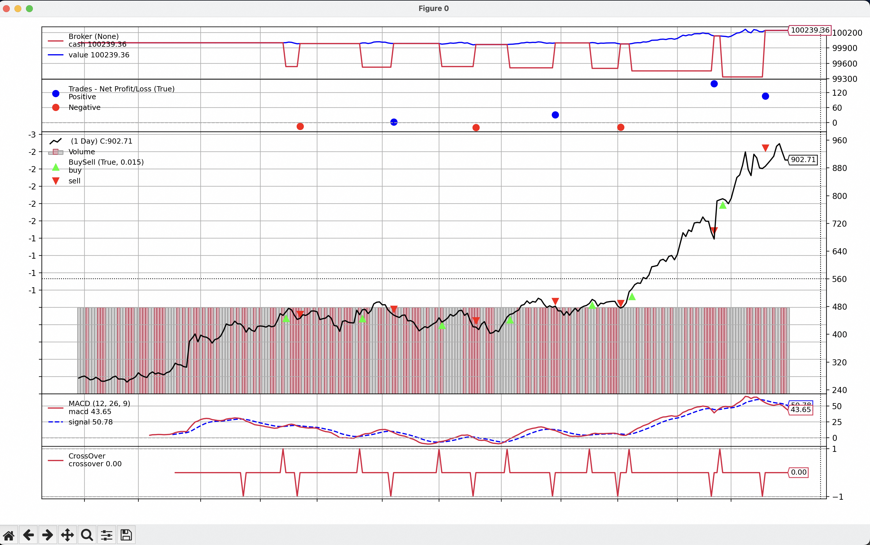
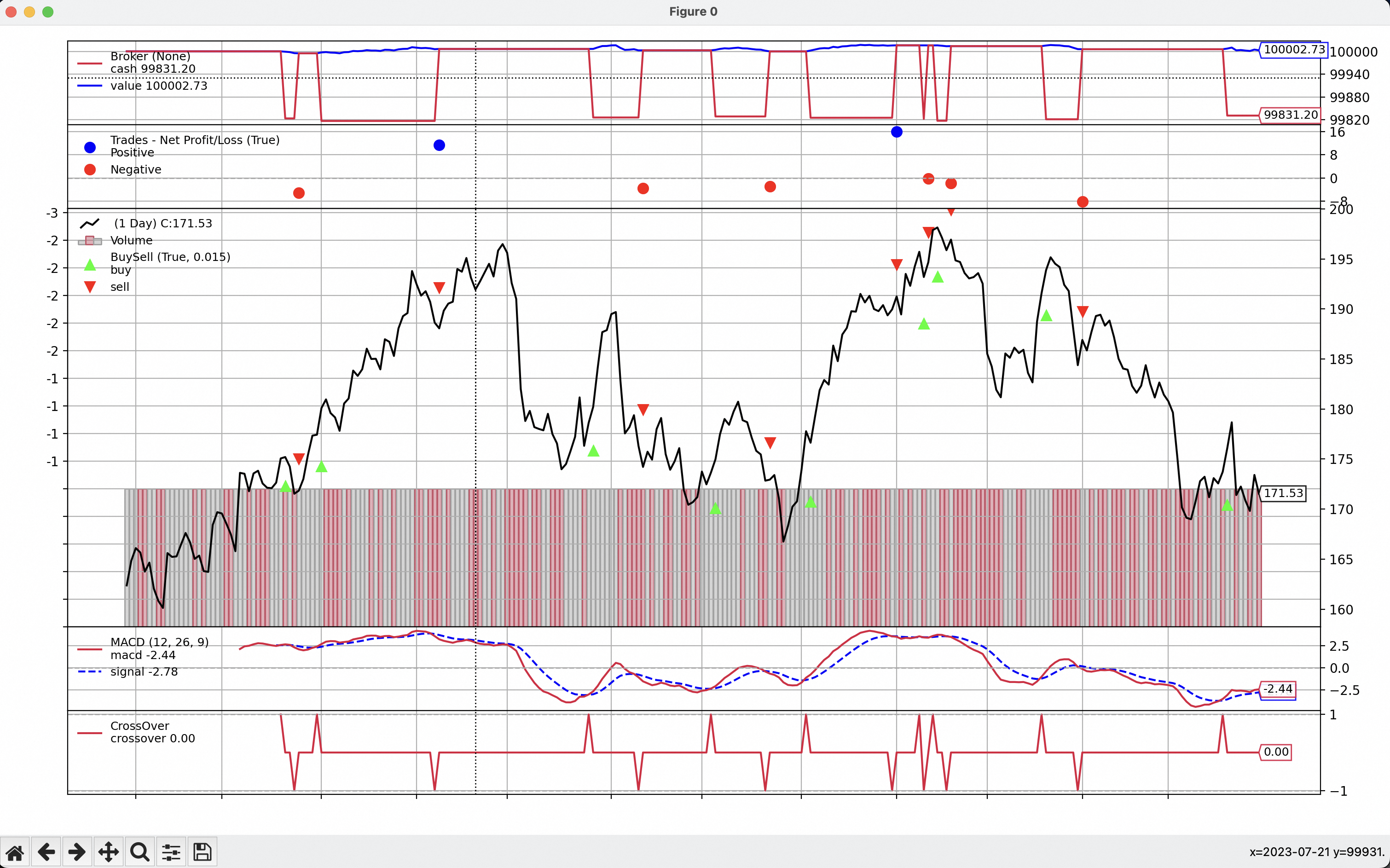
Analysis
It appears that a monotonic uptrend yields positive returns, whereas frequent fluctuations leave the principal mostly unchanged.
Enhanced MACD Strategy
GPT-4
From the simple MACD strategy code above, we noticed that it executes all-in buy and sell orders whenever a golden cross or death cross occurs.
So I posed this question to GPT-4 to see how it would solve it.
I ran this strategy, but the profit is too low—possibly because it buys and sells the entire position at once. Please optimize the strategy code to achieve better profitability through appropriate position-sizing buy and sell strategies.
Code
GPT allows specifying capital allocation ratios, stop-loss/take-profit ratios, and profit thresholds, which looks much more scientific than going all-in.
Additionally, it provides a method to search for the fast, slow, and signal parameters. You can execute it with default settings first, then check the three parameters output to the console. Next, input these parameters into cerebro.optstrategy(ImprovedMACDStrategy), for example: cerebro.optstrategy(ImprovedMACDStrategy, fast=10, slow=27, signal=5).
1 |
|
Performance
Default Parameters (12, 26, 9)
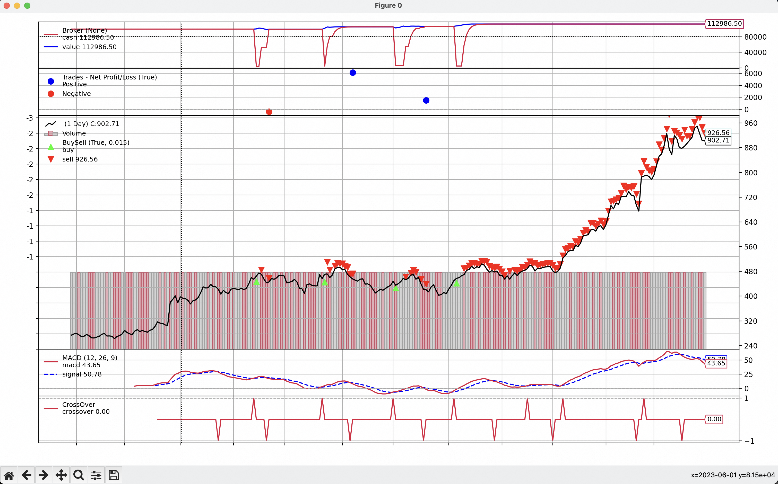
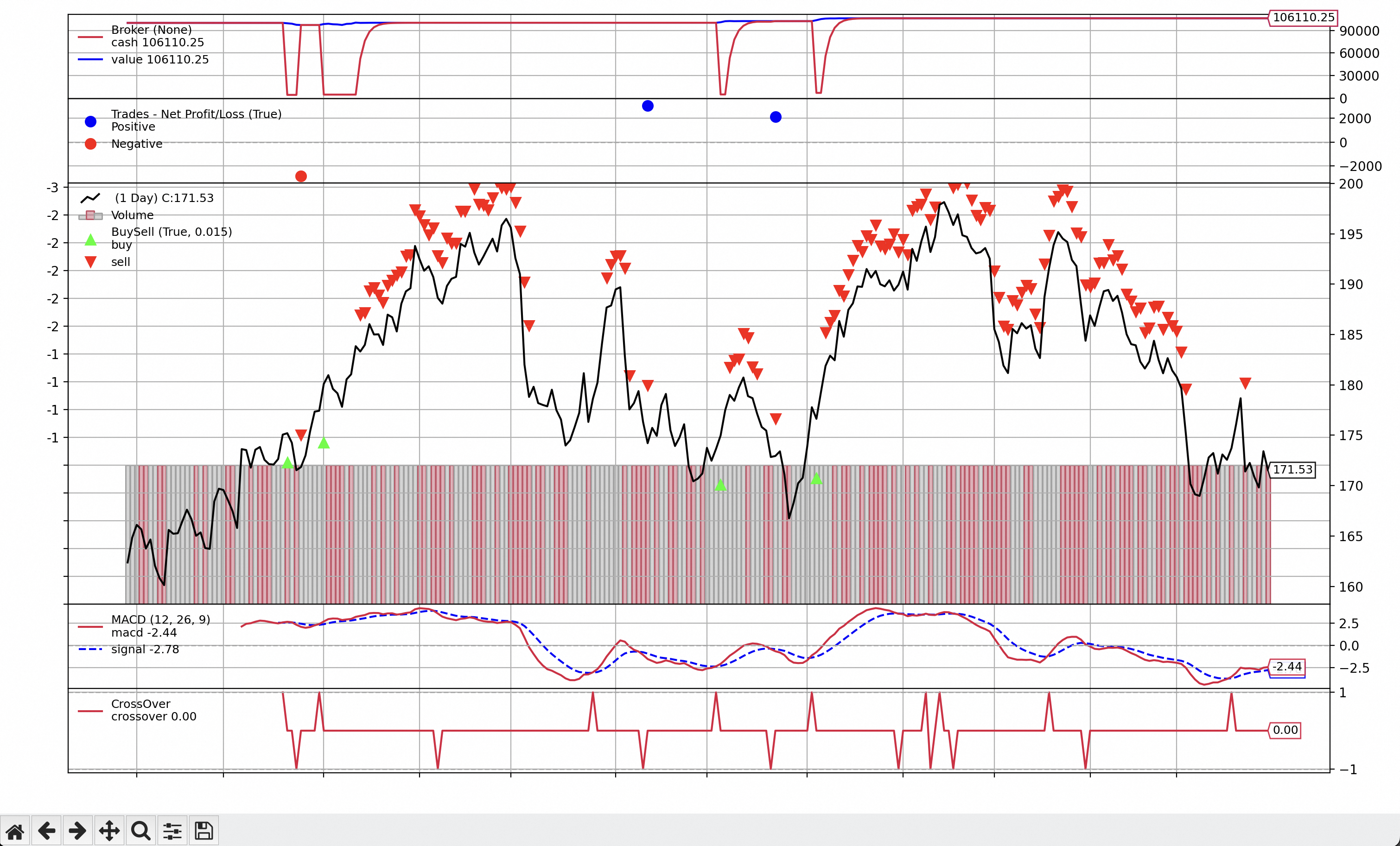
Optimal Parameters for Individual Stocks
Note: Parameters for different stocks need to be recalculated. If the market is not oscillating/range-bound, parameter calculations might not yield optimization benefits.
NVDA
Best Sharpe Ratio: 0.8460012912318833
With Parameters: Fast=13, Slow=24, Signal=9
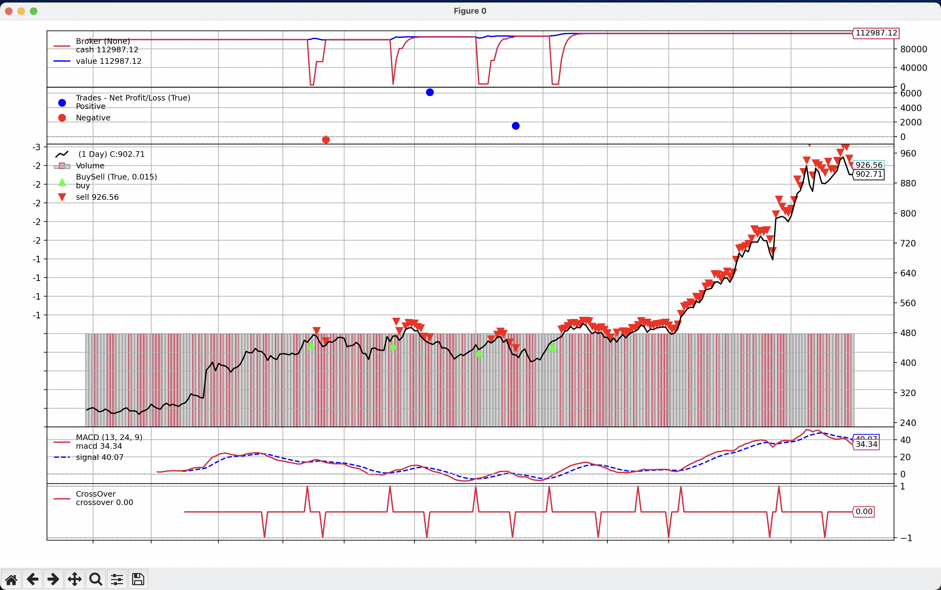
AAPL
Best Sharpe Ratio: 0.801877924498146
With Parameters: Fast=10, Slow=27, Signal=5
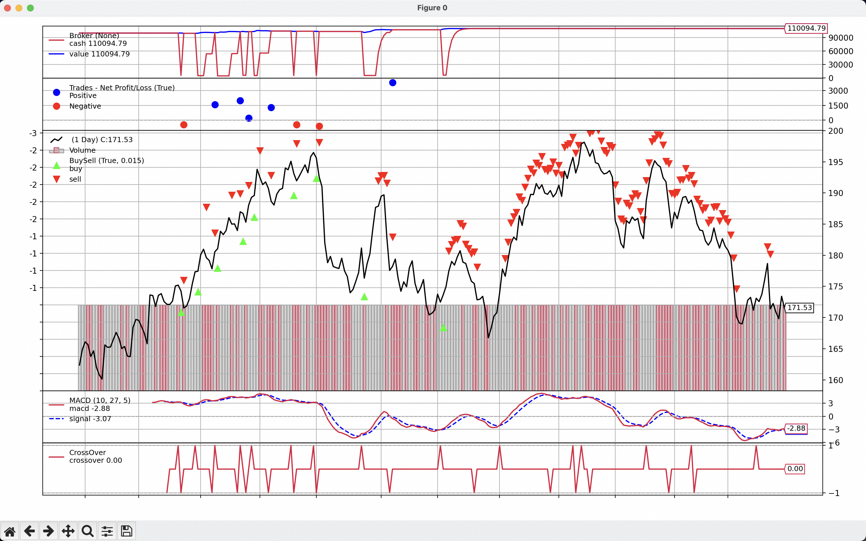
Conclusion
This article built a backtesting toolkit, introduced several common technical indicators, and provided the corresponding code and execution results.
Next, I will continue to optimize MACD and other strategies to achieve better performance.